Decision Trees in C#

Decision trees are simple predictive models which map input attributes to a target value using simple conditional rules. Trees are commonly used in problems whose solutions must be readily understandable or explainable by humans, such as in computer-aided diagnostics and credit analysis.

• Download source code
• Download sample applications
• Download the full Accord.NET Framework

Introduction

Decision Trees give a direct and intuitive way for obtaining the classification of a new instance from a set of simple rules. Because of this characteristic, decision trees find wide use in situations in which the interpretation of the obtained results and of the reasoning process is crucial, such as in computer-aided diagnostics (CAD) and in financial credit analysis. Consumer credit analysis is an interesting example because, in many countries, one can not simply reject credit without giving a justification, justification of which is trivial to extract from a decision tree.

The tree on the right has been generated using the Context Free software based on the grammar shared by davdrn.

Learning decision trees

Decision trees can be simply drawn by hand based on any prior knowledge the author may have. However, their real power becomes apparent when trees are learned automatically, through some learning algorithm.

The most notable and classics examples to decision tree learning are the algorithms ID3 (Quinlan, 1986) and the C4.5 (Quinlan, 1993). Both are examples of greedy algorithms, performing local optimum decisions in the hope of producing a most general tree. Such algorithms are based on the principle of the Occam's razor, favoring simpler or smaller trees in the hope that such smaller trees could retain more generalization power. This preference is formalized through the specification of an hypothesis ordering criteria such as the information gain. The information gain measures the, as the name implies, gain of information in using each of the attributes as a next factor to consider during decision. The information gain can be defined as:

However, the information gain has a bias towards attributes with a high number of possible values (Mitchell, 1997). A way to overcome this bias is to select new selection attributes based on alternative criteria, such as the gain ratio (Quinlan, 1986), defined as:

In the GainRatio, the SplitInformation term attenuates the importance given to attributes with many, uniformly distributed, possible values.

Iterative Dichotomizer 3 (ID3)

The algorithm presented below is a slightly different version of the original ID3 algorithm as presented by Quinlan. The modifications are to support multiple output labels. In each recursion of the algorithm, the attribute which bests classifiers the set of instances (or examples, or input-output pairs, or data) is selected according to some selection criteria, such as the InfoGain or the GainRatio.

• ID3(instances, target_attribute, attributes)
  • Create a new root node to the tree.
  • If all instances have the target_attribute belonging to the same class c,
    • Return the tree with single root node with label c.
  • If attributes is empty, then
    • Return the tree with single root node with the most common label of the target_attribute in instances.
  • Else
    • A ← the attribute in attributes which best classifies instances
    • root decision attribute ← A
    • Foreach possible value v_i of A,
      • Add a new ramification below root, corresponding to the test A = v_i
      • Let instances_vi be the subset of instances with the value v_i for A
      • If instances_vi is empty then
        • Below this ramification, add a new leaf node with the most common value of target_attribute in instances.
      • Else below this ramification, add the subtree given by the recursion:
                ID3(instances_vi, target_attribute, attributes – { A })
  • End
• Return root

Difficulties and disadvantages of decision tree learning

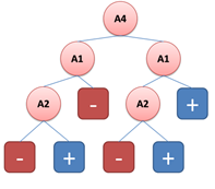
Despite relying on the Occam’s Razor to guide the learning, neither ID3 or C4.5 algorithms are not guaranteed to produce the smaller or more general tree possible. This happens because their learning is based solely on heuristics and not in truly optimality criteria. The following example, from (Esmeir & Markovitch, 2007) illustrates the learning of the concept xor (exclusive or) by the ID3 algorithm. In this example, A3 and A4 are irrelevant attributes, having absolutely no influence on the target answer. However, yet being irrelevant, ID3 will select one of them to belong to the tree. In fact, ID3 will select the irrelevant attribute A4 to be the root of the learned tree.

A1 A2 A3 A4 label 1 0 0 1 + 0 1 0 0 + 0 0 0 0 - 1 1 0 0 - 0 1 1 1 + 0 0 1 1 - 1 0 1 1 +

One complication of decision tree learning is that the problem to find the smaller consistent tree (in the sense of classifying correctly all training samples) is known to be NP-complete (Hyafil & Rivest, 1976). Moreover, the separating decision surface generated by such trees are always formed by parallel cuts alongside the attribute space axis, which could be a severely suboptimal solution (Bishop, 2007, p. 666). The example given by Bishop illustrates well this problem: for example, to separate classes whose optimum decision margin are on 45 degrees from one of the axis, it will be needed a high number of parallel cuts in comparison with a single cut on the diagonal such as could be given by any linear decision machine. Another disadvantage of traditional decision tree learning algorithms is that most methods require only a constant learning time, and, as such, do not allow for trading extra training time for a better solutions. The work of (Esmeir & Markovitch, 2007) is dedicated to overcome such problem.

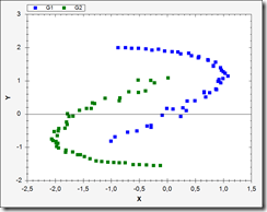
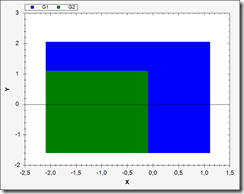
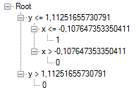
The following picture shows an example on how learning by decision trees is limited to cuts parallel to the axis, as described by Bishop. The Ying-Yang classification problem is a classical example of a non-linearly separable decision problem. Decision trees, albeit not being linear classifiers, have difficulty classifying this set with simple thresholds.

Top-Left: Ying-Yang non-linear classification problem. Top-Right: Decision surface extracted by a decision tree. Bottom: Decision threshold rules extracted from the tree.

However, despite all of those shortcomings, decision trees plays major roles as base of many successful algorithms. One interesting application and of notorious success is given in the field of object detection in images. The first real-time face detecting algorithm (Viola & Jones, 2001) is based on a degenerated decision tree (also known as a cascade). The body recognition and segmentation algorithm used by the Xbox 360 gaming platform used to process depth images generated by its companion sensor Kinect is equally based on the use of decision trees (Shotton, et al., 2011). As well is the case of the FAST algorithm for interest point detection in images (Rosten & Drummond, 2006).

I should also make the note that both the Viola-Jones and the FAST algorithms are available in the Accord.NET Framework for immediate use (the Viola-Jones (HaarObjectDetector) has also been recently updated to support multiple threads, so feel free to take a look and experiment with it!).

In sum, its possible to say that great part of the applicability of decision trees came from the simple fact that they are extremely fast to evaluate. One of the reasons for this feature is being easily translated to sets of conditional instructions in a conventional computer program. The decision trees now available in the Accord.NET Framework make full use of this fact and enables the user to actually compile the decision trees to native code on-the-fly, augmenting even more its performance during classification.

Source code

The code presented in this section is actually part of the Accord.NET Framework. The Accord.NET Framework is a framework extension to the already very popular AForge.NET Framework, adding and providing new algorithms and techniques for machine learning, computer vision and even more.

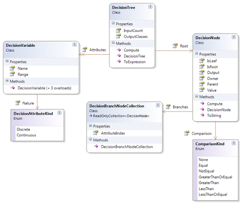
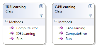
The Accord.MachineLearning.DecisionTree namespace is comprised of the following classes:

• DecisionTree, the main class representing a decision tree, with methods such as Compute to compute the tree classification given an input vector;
• DecisionNode, the node class for the decision tree, which may or may not have children nodes contained under a collection of children represented by a DecisionBranchNodeCollection;
• DecisionVariable, a class to specify the nature of each variable processable by the tree, such as if the variable is continuous, discrete, which are their expected or valid ranges;
• DecisionBranchNodeCollection, a class to contain children nodes together with information about which attribute of the data should be compared with the child nodes during reasoning.

Whose relationships can be seen in the following class diagram:

The learning algorithms available are either the ID3 algorithm discussed above, or its improved version C4.5 (which can handle continuous variables, but at this time does not yet support pruning), both proposed and published by Ross Quinlan.

Despite the bit complicated look, usage is rather simple as it will be shown in the next section.

Using the code

Consider, for example, the famous Play Tennis example by Tom Mitchell (1998):

  DataTable data = new DataTable("Mitchell's Tennis Example");
  
  data.Columns.Add("Day", "Outlook", "Temperature", "Humidity", "Wind", "PlayTennis");
  
  data.Rows.Add(   "D1",   "Sunny",      "Hot",       "High",   "Weak",    "No"  );
  data.Rows.Add(   "D2",   "Sunny",      "Hot",       "High",  "Strong",   "No"  ); 
  data.Rows.Add(   "D3",  "Overcast",    "Hot",       "High",   "Weak",    "Yes" );
  data.Rows.Add(   "D4",   "Rain",       "Mild",      "High",   "Weak",    "Yes" ); 
  data.Rows.Add(   "D5",   "Rain",       "Cool",     "Normal",  "Weak",    "Yes" ); 
  data.Rows.Add(   "D6",   "Rain",       "Cool",     "Normal", "Strong",   "No"  ); 
  data.Rows.Add(   "D7",  "Overcast",    "Cool",     "Normal", "Strong",   "Yes" );
  data.Rows.Add(   "D8",   "Sunny",      "Mild",      "High",   "Weak",    "No"  );  
  data.Rows.Add(   "D9",   "Sunny",      "Cool",     "Normal",  "Weak",    "Yes" ); 
  data.Rows.Add(   "D10", "Rain",        "Mild",     "Normal",  "Weak",    "Yes" ); 
  data.Rows.Add(   "D11",  "Sunny",      "Mild",     "Normal", "Strong",   "Yes" );
  data.Rows.Add(   "D12", "Overcast",    "Mild",      "High",  "Strong",   "Yes" ); 
  data.Rows.Add(   "D13", "Overcast",    "Hot",      "Normal",  "Weak",    "Yes" ); 
  data.Rows.Add(   "D14",  "Rain",       "Mild",      "High",  "Strong",   "No"  );

In the aforementioned example, one would like to infer if a person would play tennis or not based solely on four input variables. Those variables are all categorical, meaning that there is no order between the possible values for the variable (i.e. there is no order relationship between Sunny and Rain, one is not bigger nor smaller than the other, but are just distinct). Moreover, the rows, or instances presented above represent days on which the behavior of the person has been registered and annotated, pretty much building our set of observation instances for learning.

In order to try to learn a decision tree, we will first convert this problem to a more simpler representation. Since all variables are categories, it does not matter if they are represented as strings, or numbers, since both are just symbols for the event they represent. Since numbers are more easily representable than text string, we will convert the problem to use a discrete alphabet through the use of a codebook.

A codebook effectively transforms any distinct possible value for a variable into an integer symbol. For example, “Sunny” could as well be represented by the integer label 0, “Overcast” by “1”, Rain by “2”, and the same goes by for the other variables. So:

  // Create a new codification codebook to 
  // convert strings into integer symbols
  Codification codebook = new Codification(data);

Now we should specify our decision tree. We will be trying to build a tree to predict the last column, entitled “PlayTennis”. For this, we will be using the “Outlook”, “Temperature”, “Humidity” and “Wind” as predictors (variables which will we will use for our decision). Since those are categorical, we must specify, at the moment of creation of our tree, the characteristics of each of those variables. So:

  DecisionVariable[] attributes =
  {
    new DecisionVariable("Outlook",   3), // 3 possible values (Sunny, overcast, rain)
    new DecisionVariable("Temperature", 3), // 3 possible values (Hot, mild, cool)  
    new DecisionVariable("Humidity",    2), // 2 possible values (High, normal)    
    new DecisionVariable("Wind",        2)  // 2 possible values (Weak, strong) 
  };

  int classCount = 2; // 2 possible output values for playing tennis: yes or no

Let's now proceed and create our DecisionTree:

  DecisionTree tree = new DecisionTree(attributes, classCount); 

Now we have created our decision tree. Unfortunately, it is not really very useful, since we haven't taught it the problem we are trying to predict. So now we must instantiate a learning algorithm to make it useful. For this task, in which we have only categorical variables, the simplest choice is to use the ID3 algorithm by Quinlan. Let’s do it:

  // Create a new instance of the ID3 algorithm
  ID3Learning id3learning = new ID3Learning(tree);
  // Translate our training data into integer symbols using our codebook:
  DataTable symbols = codebook.Apply(data); 
  int[][] inputs  = symbols.ToIntArray("Outlook", "Temperature", "Humidity", "Wind"); 
  int[]   outputs = symbols.ToIntArray("PlayTennis").GetColumn(0);
  // Learn the training instances!
  id3learning.Run(inputs, outputs); 

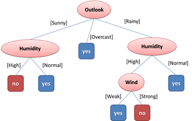
At this point, the tree has been created. A suitable representation of the learned tree could be given by the following diagram:

However, more than just a diagram, we can also go and generate a .NET Expression Tree describing our decision tree. Expression trees represent code in the form of a tree of expressions, which can then be read, modified or compiled. By compiling the DecisionTree's expression, we are able to generate code on-the-fly and let the JIT compile it down to native code at runtime, greatly improving the performance of our decision tree:

  // Convert to an expression tree
  var expression = tree.ToExpression();
 
  // Compiles the expression to IL
  var func = expression.Compile();

And here is the resulting C# code obtained by compiling the expression into a lambda function, dumping the function into an dynamic assembly, opening and inspecting this assembly using ILSpy:

  public static int Compute(double[] input)
  {
    if (input[0] == 0.0)
    {
      if (input[2] == 0.0)
      {
        return 0;
      }
      if (input[2] == 1.0)
      {
        return 1; 
      } 
      throw new ArgumentException(
        "Input contains a value outside of expected ranges.", "input");  
    }
    else 
    {
      if (input[0] == 1.0) 
      {    return 1; 
      } 
      if (input[0] != 2.0) 
      { 
        throw new ArgumentException(
          "Input contains a value outside of expected ranges.", "input");
      }
      if (input[3] == 0.0)
      {  
        return 1;   
      } 
      if (input[3] == 1.0) 
      {
        return 0; 
      }
      throw new ArgumentException(
        "Input contains a value outside of expected ranges.", "input");
    }
  }

I suspect I should have included more input validation on the generated code. However, the release is now closed and will be made available for download soon. If there is need, more robust code generation may added as a feature in later versions.

Conclusion

Decision trees are useful tools when the problem to be solved needs to be quickly interpreted and understood by humans. Another suitable use is when the decision needs to be fast. However, decision trees, at least those trained by simple training algorithms such as ID3 and C4.5 can perform quite poorly depending on the problem. As it happens with all machine learning techniques, it is futile to believe there is a one true classifier which would act perfectly on all possible imaginable scenarios. As always, it is important to know our tools and know in which situation each technique would work better.

References

• Bishop, C. M., 2007. Pattern Recognition and Machine Learning (Information Science and Statistics). 1st ed. 2006. Corr. 2nd printing ed. s.l.:Springer
• Fayyad, U. M. & Irani, K. B., 1992. On the Handling of Continuous-Valued Attributes in Decision Tree Generation. Machine Learning, January, 8(1), pp. 87-102.
• Quinlan, J. R., 1986. Induction of decision trees. Machine Learning, 1(1), pp. 81-106.
• Quinlan, J. R., 1993. C4.5: Programs for Machine Learning (Morgan Kaufmann Series in Machine Learning). 1 ed. s.l.:Morgan Kaufmann.
• Shotton, J. et al., 2011. Real-Time Human Pose Recognition in Parts from Single Depth Images. s.l., s.n.
• Viola, P. & Jones, M., 2001. Robust Real-time Object Detection. s.l., s.n.
• Mitchell, T. M., 1997. Decision Tree Learning. In:: Machine Learning (McGraw-Hill Series in Computer Science). s.l.:McGraw Hill.
• Mitchell, T. M., 1997. Machine Learning (McGraw-Hill Series in Computer Science). Boston(MA): WCB/McGraw-Hill.
• Esmeir, S. & Markovitch, S., 2007. Anytime Learning of Decision Trees. J. Mach. Learn. Res., May, Volume 8, pp. 891-933.
• Hyafil, L. & Rivest, R. L., 1976. Constructing Optimal Binary Decision Trees is NP-complete. Information Processing Letters, 5(1), pp. 15-17.

Source:http://crsouza.blogspot.com/2012/01/decision-trees-in-c.html